- How do self-serve customers from Q1 2024 behave by month 6?
- What’s the cumulative revenue impact of our March enterprise cohort?
- Where is growth accelerating or tapering across segments?
- Data source configuration: Cohorts are typically made up of many individual entities—like deals from a CRM or users from a database. To fully leverage this data in Runway, some setup is required.
- Granularity: Instead of tracking individual rows or events, cohort models group data into time-based cohorts and analyze patterns across those cohorts.
- Relative timing: Most modeling in Runway is calendar-based (month-by-month). With cohort modeling, assumptions are often made on a relative timeline—for example, 3 months after a cohort’s start.
- Import raw CRM-style data into a Source data database
- Structure your cohorts using drivers and dimensions in a Cohorts database
- Set up and apply cohort-based assumptions in an Assumptions database
- Roll everything up into a Consolidated cohort overview to see the full picture
Step 1: Bringing in CRM data into a source data database
If you’re importing already-cohorted data from external sources like Snowflake or BigQuery, you won’t need to segment by dimensions like “customer name.” To configure a new source data database:Drivers
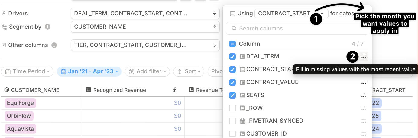
- Select the column that indicates the month when values for a given deal should start applying.
-
Check the columns containing numbers or dates you plan to use in your model.
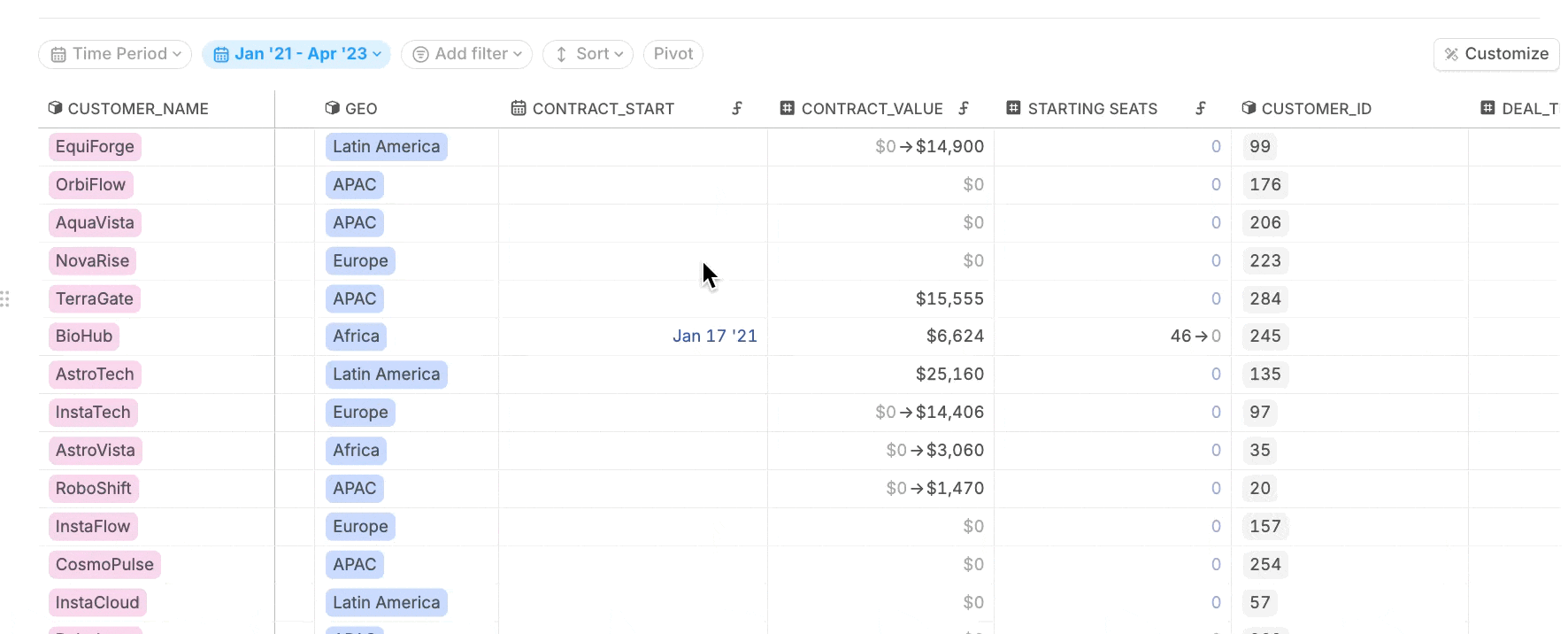
We recommend enabling “Most Recent Value” — this ensures values continue to apply in future months beyond the start month. Read more about filling sparse data here.
Segment by and Other columns
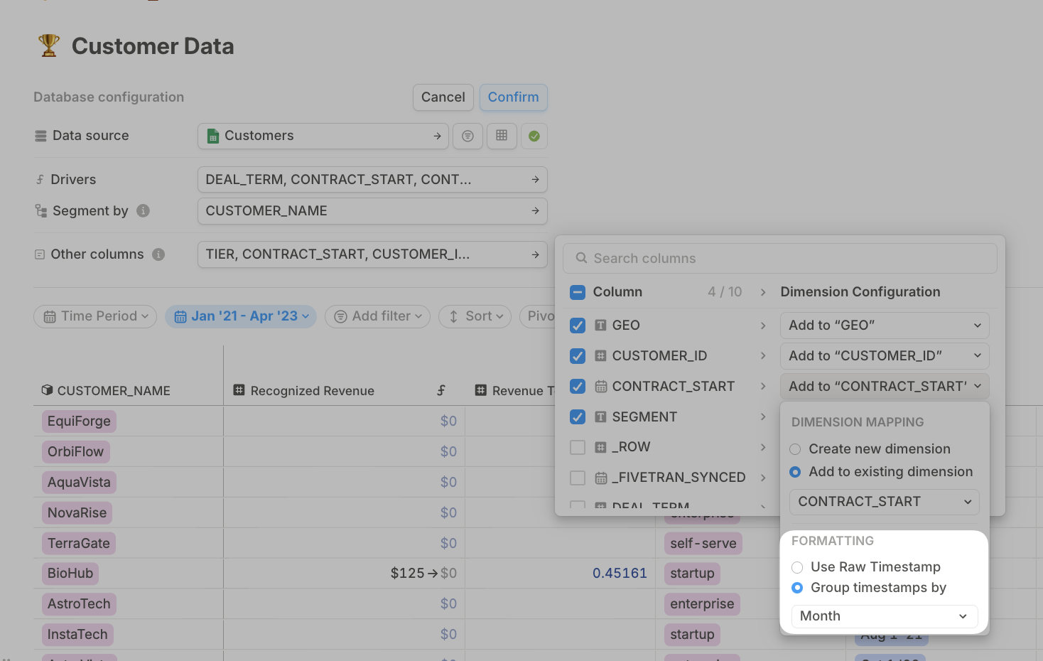
- Segment by the most detailed dimension you expect to drill into:
- If that’s customer name, make sure to:
- Add any supporting metadata in the Other columns section (e.g. sales owner, contract type).
- Add the cohort start date as an Other column — this helps with rollups in the next step.
- If your cohort start dates vary within a month, you’ll see an option to group timestamps by month (or another timeframe).
- If you’re working with pre-grouped cohorts (e.g. without individual deal visibility or with too many deals to break out), segment by the cohort start month:
- You can group assorted cohort dates by month or other units if needed.
- If you want to split cohorts further by other dimensions (like product line, region, or contract type), select those as additional Segment by options.
- If that’s customer name, make sure to:
- Use Other columns to bring in any extra metadata you want available in the model.
- Once your configuration looks good, press Confirm.
Step 2: Configuring formulas on source data
The next step is making sure your cohort data is modeled correctly across time — especially for numbers that extend into future months.-
Apply forecast formulas to match actuals where needed.
If your cohort data includes values extending into the future (e.g. pipeline data), copy the actuals formula into the forecast for your driver columns.
This ensures that the “Most Recent Value” is carried forward even beyond the Last Close.
- Use Timeseries view to manage formulas. Switch your database view under Customize > View as > Timeseries to easily manage formulas across all drivers and trace how values flow from one driver to the next. → Learn more about Timeseries view
Step 3: Setting up cohorts database
In this step, you’ll group your source data by cohort so you can model at the cohort level and track trends over time. Steps:- Create a new database This will show one segment per cohort. A name like Cohort Model works well.
-
Configure the source
Point the cohort database to the one holding your individual customer or deal-level data.
If you’re importing already-cohorted data directly from a data warehouse (e.g. via Snowflake or BigQuery), select the appropriate integration query as your source instead of referencing another Runway database.
-
Drivers - Bring in the cohort start month as a driver — this allows for time-based modeling.
- Include any drivers you want to aggregate and model at the cohort level, such as:
Seats,Contract value,Revenue.
- Include any drivers you want to aggregate and model at the cohort level, such as:
-
Segment by
- Select the dimension that defines cohort start (e.g.
Contract Start). - Add any other dimensions you’d like to separate cohorts by (e.g.
Geo,Product Line,Contract Type).
- Select the dimension that defines cohort start (e.g.
-
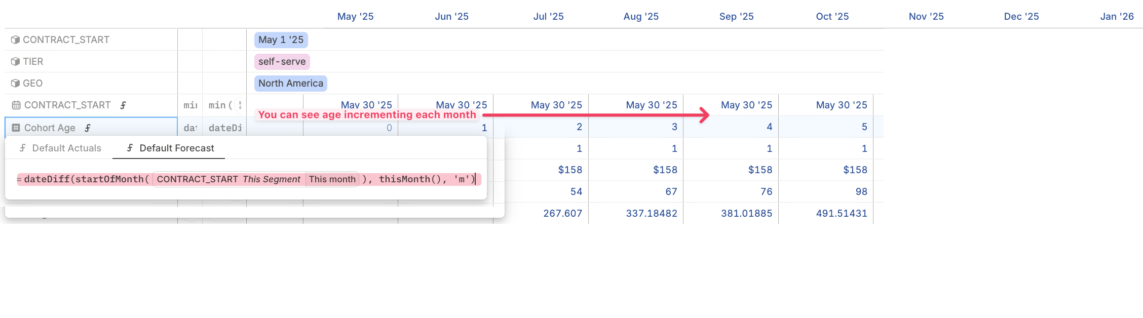
Add a driver for cohort age
This driver calculates the number of months since each cohort started. It allows you to apply the right assumptions in the right month based on cohort age.
-
Add drivers for key cohort metrics
If there are parts of your model (like churn rate, expansion revenue, etc.) that aren’t available in the source data:
- Add placeholder drivers now so that each cohort/segment has everything needed for forecasting. You can leave formulas blank for now — you’ll connect them to assumptions in the next step.
- Optional: If you want more granularity or plan to drill into these metrics, you can create them in the source data database and roll them up via the cohort database configuration. Just keep in mind that approach may be less ideal for high-level forecasting.
Step 4: Setting up cohort assumptions database
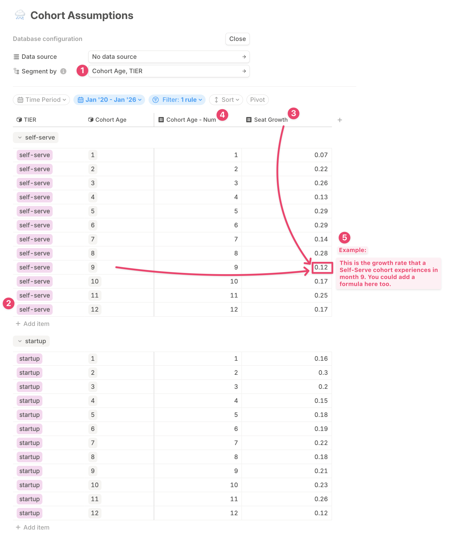
In this example, we’ll create a database to hold the assumptions that drive your cohort model — specifically, Seat growth rate as a function of both Cohort age and Customer tier. Here’s how to set it up:-
Create a new database and segment it by:
- Cohort Age (as a dimension)
- Tier (e.g. contract tier, customer segment)
- Add rows for each combination For each unique combination of age and tier, add a row. In this example, we’ve added 12 months of assumptions for each tier.
- Add a driver column for the growth rate This is where you’ll enter assumption for the expected seat growth for each cohort over time.
-
Add a numerical version of cohort age
To apply these assumptions based on a cohort’s calculated age, add an extra driver column:
- Name it Cohort Age - Number to distinguish it from the dimension.
- This enables formulas to correctly match the cohort age from your main cohort model.
-
Optional: Calculate assumptions dynamically
While the growth rates in this example are hardcoded and static across months, you can:
- Change formulas over time.
- Reference other data sources in your model to make these assumptions dynamic and responsive.
Step 5: Applying your assumptions in cohort forecasts
With both your Cohorts database and Assumptions database set up, you can now connect them to forecast key metrics — like growth in Seats — based on each cohort’s age and tier. In your Cohorts database, use the cohort’s age and the dynamic filtering capability of This Segment to fetch and apply the right assumption values for each month.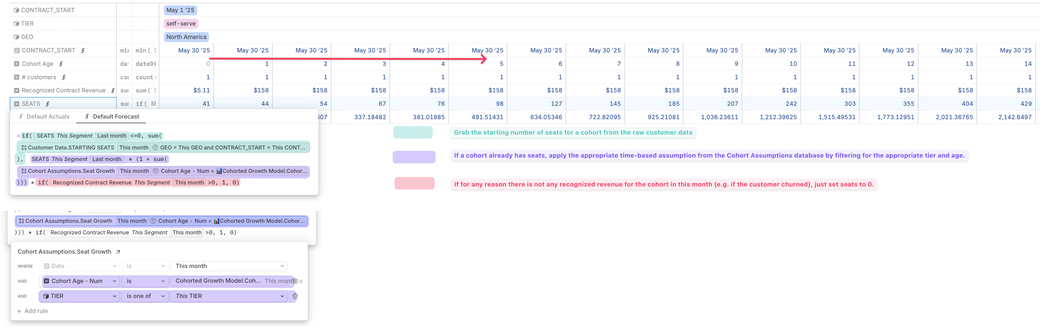
This is just one example. Your cohort model may use different logic and multiple drivers — and that’s totally supported. You can build forecasts that combine various assumptions, metrics, and time-based rules.
Step 6: Aggregating your cohorts into a consolidated overview
The final step is to create a consolidated overview — a high-level rollup of all cohorts into the segments that matter most for your business. This view makes it easy to analyze trends at a glance while preserving the ability to drill into specific cohorts and underlying customer data. Example: Summarizing by tier- Create a new database
- Set its source to your Cohort Model database
- Segment by:
Tier(or another dimension you care about) - Pull in the drivers you want to aggregate (e.g.
Seats) - Press Confirm
- The individual cohorts that contribute to each tier
- The underlying customer-level data from your source database